ATHENS, GEORGIA, 1988
Language is a wild system,
more resembling a virus
or an old-growth forest
than anything of our devising.
(Gary Snyder)
1. Introduction
2. Introduction to GPSG
2.1. Terminology of GPSG
2.2. Some critical points about GPSG
2.3. GPSG and variable word order languages
3. Properties of German
3.1. Variable word order
3.2. The noun phrase
3.3. Topicalization
3.4. Separable prefixes
4. GPSG parsing algorithms and complexity
4.1. GPSG parsing algorithms
4.2. The complexity of parsing GPSG
5. Implementation of a German grammar fragment
5.1. General description
5.2. The parsing algorithm
5.3. The generation facility and the ID-rules
5.4. The lexicon
5.5. The LP-rules
5.6. Separable-prefix verbs in the implementation
Appendix A: Examples of different parsing algorithms
(Appendices B through G are not included in the online version!)
Appendix B: Grammar and metarule application
Appendix C: The ID-rules
Appendix D: Code of the parsing algorithm
Appendix E: The LP-rules
Appendix F: The Lexicon
Appendix G: Some sample runs of the parser
Generalized Phrase Structure Grammar (GPSG; Gazdar et al. 1985) is a formal model of the syntax of natural language. Unlike earlier models such as Transformational Grammar, GPSG is confined to be context-free (CF) since CF phrase structure rules lend themselves to efficient parsing. By the mid eighties GPSG has evolved into a prominent theory. This is mostly due to two innovations. First, GPSG divides phrase structure rules into immediate dominance (ID) rules and linear precedence (LP) rules. Second, a so called slash-feature handles unbounded movements in a CF fashion. GPSG provides for a high level, compact representation of language. Because of this, it is equipped for powerful explanations of linguistic constructs but can lead to problems in computation as I will discuss further down.
A landmark in the development of GPSG was the formal specification of the complete theory by Gazdar et al. (1985). They also provided a grammar for a large set of English sentence structures. Uszkoreit (1987a) then tried to employ GPSG for German. This was an interesting endeavour in that he tried to exploit the features offered by GPSG to a language which has a high degree of word order freedom. It turned out that GPSG is well suited to accommodate word order variation.
In the meantime many efforts were made to find algorithms for effective implementations of GPSG. The first idea was to precompile GPSG into traditional CF phrase structure format. Then one could use the Earley (1970) algorithm. Shieber (1984) was the first one to propose an algorithm for direct ID/LP parsing and more sophisticated algorithms have been developed from his proposal.
This thesis tries to bridge the gap between the pure algorithmic considerations and the linguistic theories. There are on the one hand papers that deal almost exclusively with the algorithm problems. These papers are mainly concerned with the efficiency, accuracy and correctness of an algorithm for parsing ID/LP grammars (Shieber 1984; Kilbury 1984; Weisweber 1987). On the other hand we see work that is only concerned with casting constituent structures in one or the other theoretical framework without looking at ways for actually implementing these grammars (Gazdar et al. 1985; Russell 1985; Uszkoreit 1987a).
I will try to benefit from both directions. First I shall try to give an introduction into GPSG to lay the groundwork. In particular I will try to work out its advantages for parsing variable word order languages.
Then I will examine the peculiarities of the German language: the different ordering constraints in main clause and subordinate clause, the topicalization problem, and the problem of separable prefixes. The latter is a group of morphemes that have the property that they can be attached to the verb or separated from it depending on the form and the position of the verb.
In chapter 4 I will describe GPSG parsing algorithms that have been proposed to date. I will point out why I regard Weisweber's (1987) algorithm as superior. This becomes clear in contrast with the suggestions made by Evans (1987). Evans had introduced a new kind of rules to capture sisterhood information. I will show that this is a redundant notion.
My implementation is based on Weisweber's (1987) code. The grammar fragment is largely congruent with Uszkoreit's (1987a). My concern was to find a good representation of separable-prefix verbs embedded in a valid grammar for German. I will propose a way to set up a lexicon to accommodate separable-prefix entries. Special focus was also given to the integration of complex LP-rules as suggested by Uszkoreit (1987a) and to a generation component for the automatic creation of the ID/LP grammar from a given GPSG.
The program is written in Prolog and runs on a DEC VAXstation 2000 in the Advanced Computational Methods Center at the University of Georgia. Prolog allows the intensive use of unification based grammar and is therefore well suited for natural language analysis.
Although the construction of a semantic representation is central for practical purposes, this thesis is exclusively syntax oriented. May it therefore suffice to mention that GPSG generally assumes a Montague style approach which adds a semantic representation to every ID-rule. Further details can be found in Gazdar et al. (1985:182-236).
An important goal of computational linguistics has been to use linguistic theory to direct the implementation of efficient natural language processing systems. GPSG seems to be a theory that lends itself to such an implementation because of its weak CF generative power.
This chapter tries to give an introduction into the terminology and the functionality of GPSG. Space limitations compel a restriction to the very core of the framework.
GPSG contains 5 language particular components: ID-rules, metarules, LP-rules, feature cooccurrence restrictions (FCRs), and feature specification defaults (FSDs). Before we can look at these components we must clarify what syntactic categories in GPSG are and how they relate to features.
In phonology all phonemes are described by a finite set of features. Gazdar et al. (1985) suggest a similar strategy for syntactic categories in GPSG: A syntactic category is a set of feature structures. A feature structure is a pair 'feature, feature-value' where a feature-value is either an atomic value or a syntactic category. In other words, syntactic categories are "partial functions that map features to atomic feature values or to syntactic categories" (Barton et al. 1987:216). These features encode different kinds of syntactic information such as subcategorization, agreement, and unbounded dependency. The category NP is written as {[N +], [V -], [BAR 2]}. This means that it consists of the positive noun feature (N +), the negative verb feature (V -), and it is bar level 2. This feature specification for NP gets clearer when we contrast it to a VP which is written as {[N -], [V +], [BAR 2], [SUBJ -]} and a sentence S which would be encoded as {[N -], [V +], [BAR 2], [SUBJ +]}. A sentence thus differs from a VP only in containing a subject whereas both sentence and VP differ from an NP in their values for the features N and V.
Since these feature sets are somewhat long and cumbersome the GPSG literature adopts some abbreviatory conventions. The following two expressions are thus equivalent:
(1) {[N -], [V +], [BAR 2], [SUBJ -], [SUBCAT 6], [VFORM FIN]}
    =  V2[6, SUBJ -, VFORM FIN]
The number in front of the brackets specifies the bar level and the number inside refers to the subcategorization (subcat) feature. The values for the subcat-feature are arbitrarily chosen.
Gazdar et al. (1985) introduce three bar levels (0-2). Following Uszkoreit (1987a), I work with four levels to better account for the difference of sentences to VPs. The different bar values refer to the following levels:
(2) bar = 0  lexical level
    bar = 1  transition level (optional, not used with V)
    bar = 2  phrase level
    bar = 3  sentence level
This notation elucidates the close relation between NPs and VPs (N2 and V2) whereas a sentence is marked as a distinct unit by a unique bar level. Bar level 0 is usually omitted in the notation.
At this point I would like to mention that the feature notation throughout this thesis differs a little from the standard. It is based on Covington (1987). He developed a Prolog extension to accommodate feature lists of various lengths. (1) above looks like this:
(3) V2(subcat:6 :: vform:fin)The subject feature is omitted since bar level 2 now distinguishes the verb phrase from a sentence structure. Although this structure is almost self-explanatory I need to mention that it is a so called GULP feature structure which is also used in the implementation (see chapter 5). The format is (in BNF notation):
(4) GULP_Feat_Struct ::= Feature_Spec | Feature_Spec '::' Feature_Spec.
    Feature_Spec  ::= Feature_Name ':' Feature_Value.
    Feature_Value ::= GULP_Feat_Struct | Prolog_Term.
With all this in mind we can inductively specify the set of syntactic categories by listing a set of features, a set of feature values, a function that defines the range of each feature, and a set of restrictive predicates on categories (feature cooccurrence restrictions). It must be noted that categories used as feature-values can conceivably lead to recursive constructs. Therefore we need a "finite feature closure" which prevents a category Cat from being a value of feature f if Cat has f in its feature list. Figure 1 specifies the features that are used in the implementation.
 Feature     Domain             Meaning
------------------------------------------------------
 aux       {plus, minus}       modals, auxiliaries
 case      {nom, acc, dat}     nominative, accusative, dative
 compl     {nil, 'zu'}         complementizer
 dass      {plus, minus}       sub. clause starting with 'dass'
 decl      {strong, mixed,     adjective declension
            weak}
 gen       {masc, fem, ntr}    gender
 inf       SET OF VERBS        infinitive of a verb
 num       {sg, pl}            number
 pers      {1, 2, 3}           person
 prefix    SET OF PREFIXES     prefix agreement: verb to sepref
           U {nil}                 no prefix allowed
 prfst     {sep,               prefix status: separated
            att,                           attached
            insep,                         inseparable
            nopref}                        no prefix
 pron      {plus,minus}        personal pronoun
 slash     SET OF CATEGORIES   slash feature for gap handling
 subcat    {1, ..., n}         subcategorization of verb
 top       {plus, minus}       topicalized (fronted)
 vform     {bse,               bare infinitival verb form
            fin,               finite verb
            psp,               past participle verb
            pas }              passive verb
 vpos      {first, end}        verb-initial or verb-final
Figure 1: Features, their domain, and their meaning
Not all possible combinations of features make up a category. FCRs are used to formalize constraints about the cooccurrence of features in a feature list. All legal categories must satisfy all FCRs.
(5) (vpos:first) --> (vform:fin)Example (5) states that every category that has the feature-value pair 'verb position: first' must also have the pair 'verb form: finite'. This reflects the fact that every main clause must contain a finite verb. See appendix B for a complete listing of the grammar.
ID-rules closely resemble CF phrase structure (PS) rules. CF-PS rules cover dominance and precedence information whereas ID-rules only encode the dominance relation. ID-rules are of type:
(6) Cat0 --> Cat1, Cat2, ..., CatnThe left hand side (LHS) is the mother category and the right hand side (RHS) is an unordered multiset of daughter categories. Since the elements of the RHS are unordered, an ID-rule like this stands for n! traditional phrase structure rules.
LP-rules constrain the order of categories of the RHSs of ID-rules. They work only on sister categories. An LP-rule is of the form
(7) Cat1 < Cat2
meaning that Cat1 has to precede Cat2 whenever both occur as sibling constituents. Every LP-rule refers to all ID-rules.
ID/LP grammars are a subset of CF grammars. They cannot cover every construct of a CF grammar. This can easily be demonstrated with the following two CF rules which cannot be translated into ID/LP notation (Evans 1987:38):
(8) A --> B C DEvery ID/LP-grammar, on the other hand, can be translated into a CF grammar (see Kilbury 84).A --> D C B
Metarules are another important part of a GPSG. Informally, they are doing the same job as transformations in Transformational Grammar (TG). As Uszkoreit (1987a:32) puts it: "In a TG, syntactic relations among sentences are reflected in their derivational history. In a GPSG, these relations are usually reflected in the derivation of the rules that generate those sentences." Metarules have an advantage over transformations since they avoid the following implementation impasse: Transformations are mapping trees into trees. "In order to undo the transformation, we must know the structure that it produced - but we must do the parsing in order to discover the structure" (Covington et al. 1988:418).
A metarule in GPSG maps an ID-rule into an ID-rule. Metarules are formally relations between sets of ID-rules. They have a distinguished input and output pattern. If an ID-rule matches a metarule's input pattern a new ID-rule is created according to the metarule's output pattern.
(9) V2 --> X ==> V3 --> N2(case:nom), XIn (9), for every ID-rule with LHS 'V2' and some RHS 'X' we can create a new ID-rule with LHS 'V3' and the same RHS as before ('X') plus an N2 in the nominative case. Informally, this rule says that we can have a flat sentence structure whenever we have a VP.
Again we face the danger of endless recursion. Since the output of a metarule application, an ID-rule, is formally equivalent to its input, also an ID-rule, we can theoretically generate an infinite number of rules. One solution is to employ metarules within a finite closure constraint which requires that a metarule M can only be applied to a rule that did not arise from an earlier application of M. Another solution calls for the elimination of the metarule component. But abolishing it would impair the notational conciseness of GPSG. Uszkoreit (1987a:42) discusses this problem in detail.
Feature Instantiation Principles (FIPs) are means to specify category features. They include FCR, Default Value Assignment (DVA), Head Feature Convention (HFC), Foot Feature Convention (FFC), and Control Agreement Principle (CAP). Intuitively, these principles determine how feature specifications "flow" through a tree. The HFC requires the mother category to agree with its head daughter category (which has to be designated as such) in certain head features (which also have to be designated). An N2, for instance, will have the noun as its head daughter and number and person as head features. It has to agree with this daughter in number and person since these features have to match the features of a sibling V2 or V if the N2 is in the nominative case. Agreement between siblings (like subject verb agreement) can be stated in a CAP.
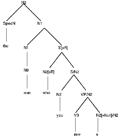
The FFP percolates foot features up from a daughter to a mother node. The most prominent foot feature is the 'slash' feature that is used to handle gaps. A WH-movement would then result in a structure like:
(10)
The 'slash' feature helps to describe context-sensitive phenomena in a CF fashion and is therefore considered one of the most important achievements of GPSG.
Gazdar et al. (1985) proposed free feature instantiation on all categories, i.e. every constituent goes through all possible instantiations of all features. Weisweber (1987:15-17) argues that this is not viable for a computational approach of GPSG since it uses too much memory. To avoid this problem, he proposes the development of a constructive procedure for feature instantiation from the static point of view of FIPs, which does not regard the FIP as a filter for local trees, but as principles of construction for the feature transportation. According to this suggestion FIPs are no longer selecting the right rules but they are now creating the right rules. In Weisweber's system feature instantiation is done while constructing syntactic structures from partial trees and local trees by unification of the root category of an admissible subtree with the daughter category of a local tree. In addition, it is done while applying feature cooccurrence restrictions.
To sum this section up, let us again look at a standard setup for GPSG and contrast it to the way I use GPSG in the implementation. GPSG has undergone considerable evolution since its introduction in the early 1980s. The current standard consists of a grammar and tree admissibility tests (Evans 1987:17):
(11)
My approach differs especially in that principle checking is integrated into the metarule extension of the ID-rules. This was made possible by applying unification based grammar. It reduces the complexity of the parser to strict ID/LP format which is computationally better understood although still not without problems.
As intriguing as GPSG might seem on first sight some caveats are appropriate. From the very start GPSG worked under the assumption that natural languages are CF. The theory was thus designed to accommodate CF languages and as we have seen is even restricted to ID/LP grammars which form a subset of CF grammars. Recently, evidence has been brought forth that suggests that human languages exceed CF language restrictions. Shieber (1985), for example, claims that Swiss German is non-CF. His argument, informally, goes as follows: Swiss German subordinate clauses can have a structure where all verbs follow all NPs (which is true, by the way, for High German subordinate clauses as well). Among such sentences there are some with more than one accusative and dative NP. The number of verbs that subcategorize for these NPs must be equal to the number of these NPs. That is, formally we get a language like:
(12) L = w a^m b^n x c^m d^n y
'a' and 'b' can be seen as the NPs in dative or accusative respectively and 'c' and 'd' are the verbs that subcategorize for these NPs. L is a classical example of a non-CF language if 'm' and 'n' range over N, the set of integers. This is the point where Shieber's proof breaks down. Although sentences in natural languages are theoretically of infinite length, in practice they never are. This means that we can find an integer i as an upper bound for 'm' and 'n' and then L is CF again.
If natural languages should finally turn out to be non-CF the framework of GPSG needs to undergo serious revision. Until that time we regard the question as an open research topic and can pursue to investigate the usefulness of GPSG for all constructs that we understand as being CF.
Because of the complication involved in understanding GPSG as a whole it is difficult to point to some of the deficiencies. Jacobson (1987) has done an intensive review of Gazdar et al. (1985) and criticizes mostly the metarule component ("a dubious complication," p. 394), the control agreement principle ("provides no general account of the fact that a VP always agrees with its s-controller," p. 398) and the unbounded dependency handling.
Metarules are seen as problematic since subcategorization is not encoded in the lexicon. The formation of passive verbs which traditionally was a lexical operation now requires metarule involvement. The slash-feature for handling unbounded dependency is a concept much praised by Jacobson. Having said this, she points to its shortcomings, mainly the fact that we cannot exclude certain structures from having constituents moved out. Jacobson (1987:390) concludes that "the ultimate contribution of GKPS [Gazdar et al. 1985], then, will probably lie not so much in the details of their particular proposals, but in the influence of their basic ideas and research program on the ongoing development of non-transformational theories of syntax."
Before proceeding I would like to anticipate two more critical aspects of GPSG that I will discuss further down. Uszkoreit (1987a) realized that an expansion of the LP-rule formalism was needed to accommodate competing ordering principles (see section 3.1.3).
Since CF languages can be parsed in polynomial time it has been claimed that GPSG can also be parsed in polynomial time. Barton et al. (1987) showed that this is not the case. They claim that the fastest recognizer for unrestricted GPSG must take exponential time or worse. They therefore propose restrictions to the formalism (see section 4.2).
The most attractive feature of GPSG for parsing variable word order languages is the ID/LP distinction. Information about dominance (ID) and precedence (LP) is separately encoded in the grammar.
Weisweber (1987:12) states that "from the point of view of a computer scientist the ID-LP distinction does not buy much." But from the linguist's point of view it is a tool to better express certain language features. It allows the linguist to make explicit statements about precedence relationships, which was not possible in traditional phrase structure grammars. It is now even possible to encode precedence information dependent on feature values (and not only on categories).
(13) X(top:plus) < V3LP-rule (13) states that every constituent with the feature 'top:plus' (which means that the category is topicalized; see section 3.3) precedes any sibling V3.
At the same time GPSG makes predictions about the degree of word order variation. Only sibling constituents can be permuted.
(14)  A --> B, C
      B --> D, E
      C --> G
These ID-rules would not allow for the string "DGE" since D and E are not adjacent to each other. Ordering phenomena that exceed constituent boundaries must be handled by category-valued feature percolation (slash-feature) or by modified constituent structures. Feature percolation is used mostly for long distance dependencies. They express certain syntactic relations like WH-gap relation.
A possible solution to accommodate ordering phenomena across constituent boundaries is the "flattening" of structures. The name relates to the flatter tree that results from these structures. An additional ID-rule like
(15) A --> D, E, G
in the above example would allow for the string "DGE" which was excluded before.
"Liberation" metarules have been introduced to create these flat structures. We can then stick to the regular constituent structure where possible and apply these liberation rules only for specific purposes. This provides for the generalization of regular structures while at the same time we are able to generate special cases. Careful LP-rule constraints have to be added to avoid undesired multiple structures after application of the liberation rules. Metarule 1 of my implementation (given in (9) above) is an example of a liberation rule. It creates a flat sentence structure to accommodate verb initial sentences. See chapter 3 and 5 for more details.
This brings us to the end of the GPSG overview. I have shown many of the ingredients of this grammar formalism although intensive study is required to fully capture the interplay of the various components. Now that we have introduced the formalism let us look at the object, that we want to formalize: the German language.
German syntax challenges the linguist in many ways. I will try to point out some peculiarities in comparison to English. The focus will be on problems relevant to my implementation. Semantic aspects will be mentioned only if they contribute to the discussion of syntactic structure.
In German we can distinguish three different clause types with respect to the position of the finite verb. There are verb-initial, verb-second, and verb-final clauses.
The verb-second clause is the most frequent and is therefore often called the basic order. In this category we have regular untopicalized assertions like (16a) and (16b). It also includes questions, that are introduced by a WH-word like (17), and atypical subordinate clauses that lack the conjunction like in (18).
(16a) Peter sieht das Buch.
      Peter sees  the book.

(16b) Heute sieht Peter das Buch.
      Today sees  Peter the book.

(17)  Wer sieht das Buch?
      Who sees  the book?

(18)  Ich weiss, du siehst das Buch.
      I   know   you see   the book.
(16b) is different from English in that the adverb in clause-initial position triggers the subject-verb inversion. The first position in a verb-second main clause can be occupied by many different constituents under different circumstances. This aspect is discussed in detail in section 3.3.
The verb-initial order is used for yes/no questions and imperatives. It can also be found with antecedents of conditions if they are not marked by particles like wenn 'when' or falls 'if' (19).
(19) Fährt Peter morgen,   dann komme ich schon   heute.
     goes  Peter tomorrow  then come  I   already today
     If Peter leaves tomorrow then I come today.
Exclamations can also be formulated with the verb in the initial position. This gives them more of a questioning character. Finally, subjunctive subordinate clauses have verbs in the first position:
(20) Peter wäre     zuhause geblieben, hätte er das Wetter erwartet.
     Peter would have at home  stayed    had  he the weather expected
     Peter would have stayed at home had he expected the weather.
The third ordering type is the verb-final type. This is the typical order for most subordinate clauses. It occurs especially when they are introduced by a conjunction, a complementizer (21), a relative pronoun, or an interrogative pronoun.
(21) Paul weiß,  daß Peter nach hause kommt.
     Paul knows that Peter to   home  comes
     Paul knows that Peter comes home.
Uszkoreit (1987a) claimed that we can capture these three clause types with two LP-rules:
(22a) v(vpos:first) <  X
(22b)       X       <  v(vpos:end)
These rules refer to the finite verb. (22a) states that a verb with the feature 'vpos:first' (a verb in a main clause) precedes every sibling whereas (22b) forces a verb into clause-final position if it has the feature 'vpos:end'.
Uszkoreit then provides two sentence structure types to accommodate verb-initial and verb-second main clauses. The first one is a flat structure that leads to the following tree. Please note that the order of the N2s is not specified by any LP-rule and can therefore be switched.
(23)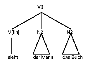
This tree does not indicate the different relations that hold between the verb and its object and subject (i.e. the VP node is missing). This is justified since a VP node would result in an entangled tree which is undesirable for parsing purposes. The traditional NP-VP distinction is often blurred in German because of the relatively free order of the verb's arguments and adjuncts.
The second sentence structure type is deeper (24). Every constituent that precedes the matrix clause is treated as being moved out of it. Thus the subject NP in clause initial position is just a special case of fronting.
(24)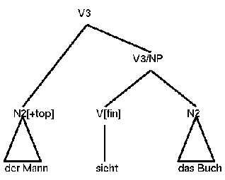
The order of the fronted constituent (which gets the feature 'top:plus') and the matrix clause is specified by an LP-rule.
(25) X(top:plus) < V3This requires that every fronted constituent precedes the sibling sentence.
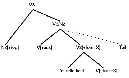
In a subordinate clause the verb has to be in final position (except for some subjunctive cases which we can treat as main clauses). We could get both of the above structures as subordinate clause structures with the verb in final position. Since the verb complex is always united at the end of the sentence the 'slash' structure is not needed. We can reserve it for main clauses.
According to Engel (1977:192), the German main sentence is arrayed by a "clause-frame". He explains that the verbs of the main clause open up this frame and divide the clause into headfield, middlefield, and tailfield (26). The constituents of the headfield as well as the finite verb have to always be present. Every other field is optional.
(26)
    Headfield | Finite V | Middlefield | Rest of Vgroup  |  Tail
       Ich       habe      mehr          gesehen          als ihr
       I         have      more          seen            than you
       I have seen more than you.
The tailfield usually contains constituents that we could have equally well
added to the middlefield. Therefore the tail is often empty. Note that the
above LP-rules do not specify the position of the rest of the verb group. In my
implementation I therefore assume that the middlefield and the rest of the verb
group form a V2 which I declare to have subordinate clause structure while at
the same time I ignore the tailfield. I then get a structure like this:
(27)
The order in the verb group is determined by a dependence relation. The dependent verb always goes to the left of the head verb with the exception of the finite verb which is moved to the initial position of the clause core in main clauses. The dependence-relation is defined as: A verbal element VE1 is the head verb of another verbal element VE2 if VE1 determines the morphological form of VE2. For example, the finite verb is the head verb of the nonfinite verb, the modal verb is the head verb of the full verb, etc. For a formal description of this relation, please consult Engel (1977:114-118). The order of the German verb group is thus a mirror image of the English order (Uszkoreit 1987a:15).
Uszkoreit's LP-rule (22b) forces the finite verb into the final position in a subordinate clause. In addition to the exception of subjunctive subordinate clauses, which require special treatment, we also need to consider the ordering problem of complex verb structures. In most cases Uszkoreit's setup, which follows the dependence relation, is correct even for complex verb sequences like (28). In a subordinate clause like (29), however, the finite verb necessarily precedes the nonfinite verbs.
(28) ... weil  Peter gesehen worden sein könnte.
         since Peter seen    been   have could
     ... since Peter could have been seen.

(29) ... weil  Peter hatte getragen werden dürfen.
         since Peter have  carried  been   may
     ... since Peter may have been carried.
To understand this phenomenon we need to look closer at the different types of verbs that are involved in the above examples. Engel (1977:112) classifies the German verbs into 6 groups for this purpose:
e.g. schneiden 'cut', stützen 'support', erscheinen 'appear'.
haben 'have', sein 'be' (in connection with psp forms).
dürfen 'may', können 'can', mögen 'may', müssen 'must', sollen 'should', wollen 'want' (in connection with bse forms).
e.g. anfangen 'start', belieben 'love', pflegen 'used to', scheinen 'seem', verstehen 'understand' (in connection with zu + infinitive).
Many verbs in this group can also be used as "full verbs". Sometimes they change their meaning.
e.g.
"Die Sonne scheint."  vs  "Er scheint zu schlafen."
 The  sun  is shining.     He seems   to sleep.
Some verbs in this class take a regular infinitive (without zu), e.g. lassen 'let'.
kommen 'come', bekommen 'get', kriegen 'get'
(in connection with the past participle of another verb).
e.g.:
Er bekommt es gesagt.
he gets    it said
He is told it.
e.g. ab, an, auf, aus, bei, ...
Figure 2: Classification of verbal elements (Engel 1977:122-114)
The following rule captures the regularity (Engel 1977:117): If the verb complex contains a non-finite modal verb or a modality verb of type 4.2 then the finite verb is moved to the front of the verb complex.
The reason for the finite verb movement in subordinate clauses is not clear. Many ordering principles seem to be influenced by stack considerations. A speaker chooses the order that requires the least amount of mental work. Although this consideration might influence the above explained shifting of the finite verb it cannot be the only reason. Some clauses are still grammatical even if the finite verb is in the final position of a four-verb complex (see example 28). On the other hand, there is some evidence that it is a disambiguation precaution. The striking modal verbs and modality verbs (type 4.2) have the same forms for the infinitive and the participle. The finite verb in front of the complex indicates that only the participle reading is appropriate.
Sentence (30) allows all six permutations of its noun phrases without a significant change in meaning.
(30) Der Junge    gibt   dem Mann      das Buch.
     NP(case:nom)        NP(case:dat)  NP(case:acc)
     the boy      gives  the man       the book
     The boy gives the book to the man.

     Der Junge    gibt   das Buch      dem Mann.
     Dem Mann     gibt   der Junge     das Buch.
    ?Dem Mann     gibt   das Buch      der Junge.
    ?Das Buch     gibt   dem Mann      der Junge
     Das Buch     gibt   der Junge     dem Mann.
Some of these permutations are stylistically strange, but they are all acceptable German sentences. This changes as soon as pronouns are involved. In (31) the pronoun (NP(case:acc)) has to precede the NP(case:dat). Therefore (31) is not acceptable.
(31) *Der Junge     gibt   dem Mann      es.
      the boy       gives  the man       it
      NP(case:nom)         NP(case:dat)  NP(case:acc)
Uszkoreit (1987a:18-24 and 113-127) explores some of the regularities that underlie the order of the verbal arguments. He found constraints on the phonological, syntactic, and pragmatic levels.
He includes "heavy NP-shift" (for English) as one of the phonological constraints. A heavy NP displays a high degree of internal complexity. Such an NP occurs preferably at the end of a sentence even if the resulting sequence deviates from the standard order. In German we notice a similar phenomenon: a shorter constituent precedes a longer one ("das Gesetz der wachsenden Glieder"). I believe that these two principles are performance constraints rather than phonological rules. They can easily be explained with the "mental stack" theory.
Taking the computer paradigm to explain language understanding, we assume that on parsing, every word together with its special features is pushed into a "mental" stack. Whenever a phrase is parsed its words are removed from the stack and the semantic representation of the phrase is pushed in. This continues until a meaningful unit is created. Human beings try to keep the stack as small as possible. This is only an informal description of this process and does not claim to be proven correct.
Heavy NP-shift facilitates the stack operation by giving precedence to simple constituents which might help to understand more complex NPs by establishing most of the grammatical relations early. The same is true for the German case. If the complex NP follows the simple NP the stack does not have to hold a valence gap for a long time. To illustrate this point let us look at (32):
(32a) Ich erklärte  den Kindern  die Relativitätstheorie.
      I   explained the children the theory of relativity
      I explained the theory of relativity to the children.

(32b) ?Ich erklärte die Relativitätstheorie den Kindern.

(32c) Ich erklärte die Relativitätstheorie den Kindern meiner Klasse.
      I explained the theory of relativity to the children of my class.
While parsing (32b) the hearer knows how many NPs to expect after "analyzing" the main verb. If the first NP is complex it takes some effort to keep in mind that there is another one still to be received. Therefore we try to move complex constituents to the end. Another phonological constraint seems more plausible. Uszkoreit (1987a:23) suggests that people try to avoid a stress clash as in (33a) and would therefore rather say (33b).
(33a) (the italics indicate stress)
      Ich zeigte die Parodie Kurt.
      I   showed the parody  Kurt
      I showed Kurt the parody.

(33b) Ich zeigte Kurt die Parodie.
But I doubt that a constraint like this can be implemented in a parser unless we incorporate phonological features.
Uszkoreit's pragmatically based ordering principles include rules such as "old information precedes new information" and "relevant information follows less relevant". They are mentioned here for completeness and will not be pursued further.
Most important for my work are the syntactic ordering rules. There is some ongoing discussion about the unmarked order in German sentences. Uszkoreit proposes the order: SUBJ, IOBJ, DOBJ. This order can be overwritten if a constituent is focused or if the NP is a pronoun. To account for these competing principles, Uszkoreit expanded the traditional LP-rule formalism. He came up with a compound LP-rule:
(34)  +NOM     <  +DAT
      +NOM     <  +ACC
      +DAT     <  +ACC
      -FOCUS   <  +FOCUS
      +PRONOUN <  -PRONOUN
Usually a string is rejected if one LP-rule fails. This compound rule on the contrary is a disjunction of its atomic rules. If any of the atomic rules succeeds (or if none applies) the whole rule succeeds.
This type of rule will be useful to implement other competing principles. Although future rule systems probably ought to be able to accommodate different weights on competing principles to account for differing degrees of acceptability.
Since this thesis is mainly concerned with the correct parsing of variable word order, the composition of noun phrases is of minor importance. Noun phrases employ only a small degree of word order freedom, mostly in combination with genitive attributes so that the usefulness of an ID/LP approach is less obvious.
In German the determiner and its noun have to agree in case, number, and gender. Gender is arbitrarily assigned to every noun.
(35) das Haus    (case:nom :: num:sg :: gen:ntr)
              or (case:acc :: num:sg :: gen:ntr)
     the house

(36) den Häusern (case:dat :: num:pl :: gen:ntr)
     the houses

(37) der Zeitung (case:gen :: num:sg :: gen:fem)
     the newspaper
If the noun phrase includes an adjective phrase, it too must agree in case, number, and gender with the head noun. Furthermore the adjective must agree with a declension as prescribed by the determiner (see 38 and 39).
(38) das schöne  (decl:weak)  Haus
     the pretty               house

(39) ein schönes (decl:mixed) Haus
     a   pretty               house
We distinguish between three adjective declensions: strong, weak, and mixed. The strong declension is used after the zero determiner, or with an invariable determiner like zwei 'two'. The weak forms occur with the definite determiner (e.g. das 'the'), with demonstrative and interrogative pronouns in determiner function (e.g. dieser 'this', jener 'that', welcher 'that'). The mixed declension is applied after the indefinite determiner (e.g. ein 'a'), the negative determiner (e.g. kein 'no'), and after possessive pronouns (e.g. mein 'my'). The latter group is called 'mixed' since its endings are a mixture of the former two groups. (For a detailed treatment of adjective agreement in German, see Zwicky 1985.)
Since this is a clear division, we can accommodate it easily in the lexicon. Every determiner (the particular pronouns are listed as determiners) will have a feature 'decl' in its feature list. The value of this feature will govern the adjective declension. Every adjective is listed only once in the lexicon with its stem as word form. A morphology component computes the appropriate adjective form depending on the 'decl' value whenever needed.
Many different constituents can precede the verb in a verb-second assertion main clause. These constituents are topicalized, i.e. they are made the topic of the assertion. The following constituents can generally be fronted: the subject (40a), any object (40b), adverbial phrases (40c), adverbs (40d), predicatives (40e), and nonfinite verbs (40f).
(40a) Peter sah den Mann.
      Peter saw the man.

(40b) Den Mann sah Peter.
      Peter saw the man.

(40c) Vor einer Stunde sah Peter den Mann.
      ago one   hour   saw Peter the man
      Peter saw the man one hour ago.

(40d) Heute sah Peter den Mann.
      Today saw Peter the man
      Peter saw the man today.

(40e) Schön     ist der Garten heute.
      beautiful is  the garden today
      The garden is beautiful today.

(40f) Gesehen hat Peter den Mann.
      seen    has Peter the man
      Peter has seen the man.
All these constituents can also follow the verb and are just moved to the front for some semantic reason that I will try to specify below. In addition we have the expletive es 'it' which can only occupy the fronted position.
(41) Es kommen Tiere   aus dem Dschungel.
     it come   animals out the jungle
     It is animals that come out of the jungle.

(42) Es wird gegangen. (und nicht gefahren)
     it is   gone (walked)
     The trip is to be made on foot! (and not by car)
The expletive es appears as a substitute when no other constituent is available as with the impersonal passive in (42). Nerbonne (1984:87) calls it "zero-fronting". It should be distinguished from the supletive es as in (43a) which can also occur behind the verb (43b). It should also be differentiated from the homomorphic personal pronoun. In (44) this pronoun refers back to a noun (gender:neuter).
(43a) Es graut  mir vor dir.
      it scares me  of  you
      You scare me.

(43b) Mir graut  es vor dir.
      me  scares it of  you
      You scare me.

(44)  Es steht  in der Hauptstraße.
      It stands in the main street.
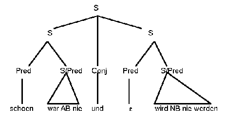
Nerbonne (1984:84ff) mentions two more fronting peculiarities. He observed that the fronted constituent can relate to both parts of a conjunction.
(45) Schön  war Alt-Bochum nie und wird Neu-Bochum nie werden.
     Pretty was Old-B    never and will New-B    never become
     Old-B was never pretty nor will New-B ever become pretty.
His interpretation would lead to the following sentence structure:
(46)
He also notes that this usage is hard to formalize. The fronted constituent in such a compound sentence can only be an NP in nominative, dative, or accusative or a predicative. I therefore suggest that this case might be treated as a fronting of both the first sentence and the second sentence with an elliptic fronted constituent for the second one. I propose sentence structure (47). Then both Ss can be handled in the same way as regular frontings in their respective clauses and we can treat the elliptic constituent as a gapping phenomenon.
(47)
Nerbonne also notes that German fronting can be unbounded. He refers to Uszkoreit (1982) who gave the following example.
(48) In dieses Zimmer sagte er, daß er den Stuhl gestellt hatte.
     in this   room   said  he that he the chair put(psp)  had
     He said that he had put the chair in this room.
Since the 'slash' feature is the only mechanism in GPSG to handle unbounded movement, the use of the 'slash' feature to handle fronting in general seems to be justified by this example.
It is noteworthy that in the majority of cases exactly one major phrasal constituent is fronted. But there are exceptions to this. It is possible to have a prepositional phrase fronted together with an object (49) or to have two prepositional phrases fronted (50). We also can have an object accompanying an infinite verb in the fronted position (51).
(49) Viel     Spaß mit  den Kindern  hatten sie.
     a lot of fun  with the children had    they
     They had a lot of fun with the children.

(50) Mit  den Hühnern ins Bett pflegte er zu gehen.
     with the chicken to  bed  used    he to go
     He used to go to bed very early.

(51) Das Buch geben will ihm der Mann.
     the book give  want him the man
     The man wants to give him the book.
Engel (1977:215) also mentions cases where a constituent is fronted together with a "quasi-attribute" (like also 'even' and andererseits 'on the other hand') or a conjunctor. These are used to emphasize the semantic function of the fronted block.
Engel (1977:216-221) proposes three semantic functions that fronting can have. First, it can be used to connect a sentence to previous text. Second, it can be used to put special focus on the constituent. Finally, in some cases, it is used for disambiguation. Engel also mentions that none of these functions is limited to the fronted constituent. The same function can also be achieved in the middlefield of the sentence by ordering, stressing, or other measures.
Many problems are involved with allowing multiple fronted constituents. Because of these problems my implementation allows only for one such constituent to be fronted. In fact, this might already be the limit that GPSG can handle. Uszkoreit (1987b) pointed out that in case of multiple fronted constituents the order of these constituents can only be determined in relation with the order of the constituents that remain in the middlefield. That means we have linear ordering constraints that cannot be handled with traditional LP-rules which work on continuous siblings only. But the LP-rules are one of the essential components of GPSG and cannot be altered without fundamentally changing the theory. Uszkoreit (1987b) proposes a more intelligent lexicon to handle the problem. Future research will show if that is a viable solution.
Separable verb prefixes are an interesting feature of the German language. As the name implies, they are either attached to their verb (52) or separated from it (53). They are thus different from inseparable prefixes that are always bound (in 54 and 55 über is an inseparable prefix of holt).
(52)  Peter hat die Post abgeholt.
      Peter has the mail up-picked
      Peter has picked up the mail.

(53)  Peter holt  die Post ab.
      Peter picks the mail up.

(54)  Peter hat das Auto überholt.
      Peter has the car  over-taken
      Peter has passed the car.

(55)  Peter überholt   das Auto.
      Peter over-takes the car
      Peter passes the car.
Wunderlich (1983) has investigated prefixes of local verbs. He believes that the following parallelism explains the origin of prefixes: "A local verb (position or movement verb) can take a local prefix. A local verb can take a local prepositional phrase." This lead him to the assumption that a prefix is the remainder of a prepositional phrase.
Wunderlich (1983:456) then proceeds to formulate the structural differences of separable and inseparable-prefix verbs. Since these remarks are concise and accurate I quote them here to provide the basis for my discussion: Let V0 be a simplex verb and P be a prefix.
(56) "The inseparable-prefix verb behaves like a normal verb; it therefore belongs to the same category V. It has the structure [P + V0]V with the following properties:
e.g. Underlying structure:
er das Bett überzieht
He puts fresh linen on the bed.
Finite-verb fronting and topicalization:
Er überzieht das Bett.
e.g. with perfect tense:
Er hat das Bett überzogen.
e.g. Er versucht, das Bett zu überziehen."
(57)
er den Vorhang aufzieht.
('he opens the curtain')
Finite verb fronting and topicalization:
Er zieht den Vorhang auf.
Er hat den Vorhang aufgezogen.
e.g. Er versucht, den Vorhang aufzuziehen."
There are some assumptions made in this definition that are worth examining. First, it is striking that Wunderlich assumes an underlying structure with the verb in final position. The notion of an underlying structure reminds us that he works within the framework of Transformational Grammar, which distinguishes between deep structure and surface structure. On the other hand this approach provides an elegant explanation of the fact that separable prefix and finite verb are separated in main clauses. According to his interpretation it is not the case that the separable prefix is taken from the verb and moved to the end. On the contrary it is true that the prefix "resisted" the verb movement and stayed at the original location. This corresponds to the observation that the position of the separable prefix is generally identical to the position of the nonfinite verb group.
Second, Wunderlich assumes that a separable-prefix verb is a unique word. The most important indication in favor of this assumption is the accent. Since the separable prefix has the word accent it must be part of the word which otherwise would not have an accent at all. This gets especially striking when we look at the infinitive form with zu (compare to 4. in the above schema). For inseparable-prefix verbs the stress is on the verb which leaves the complementizer zu as a separate word. For separable-prefix verbs the stress is on the prefix which results in the complementizer being an infix between prefix and verb. Please note that this complementizer is not to be mixed up with the prefix zu as in zubereiten 'prepare'. Here, of course, we would get the strong infinitive form zuzubereiten.
The cases in which the prefix separates from the stem depend on the clause type with respect to the position of the finite verb. Only if a finite main verb is in the second position of a clause does the prefix stay separate in the ultimate position of the clause core.
Prefixes do not change the morphology of their verbs but they do change the subcategorization. Therefore separable-prefix verbs need two kinds of entries. One of them needs to specify the subcategorization that the verb can take in combination with the prefix.
(58) subc_entry(v(subcat:Num1 :: prefix:Pref), [sehen]) :-
      member(Pref,[an, durch, ein, nach, nil]).
     ==> subcategorizes for N2(case:nom), N2(case:acc)

(59) subc_entry(v(subcat:Num2 :: prefix:auf), [sehen]).
     ==> subcategorizes for N2(case:nom)
The other one should list all the verb forms since they remain the same for every subcategorization.
(60) verb_entry(v(pers:1 :: num:sg :: vform:fin :: inf:sehen),sehe).
     verb_entry(v(pers:2 :: num:sg :: vform:fin :: inf:sehen),siehst).
     ....
     verb_entry(v(                    vform:bse :: inf:sehen),sehen).
A computing algorithm can now do the lexicon lookup and compute the necessary information (see chapter 5 for details).
The general scheme behind the subcategorization change is not known. It would be interesting to explore if the same prefix changes the subcategorization of different verbs in the same way. This is too broad a topic to be covered in this thesis and has to be left open to future research.
Inseparable-prefix verbs have a subcategorization entry like any other verb that does not take prefixes. We need to enter all the verb forms again for the inseparable-prefix case since some differ from their separable-prefix counterparts. For example, the past participle form of the inseparable-prefix verb übersetzen 'translate' is übersetzt. For the homomorphic separable-prefix verb übersetzen 'ferry across' the past participle is übergesetzt.
Uszkoreit (1987a:111) claims that prefix and verb are a lexical unit but at the same time distinct syntactic constituents. A metarule can then capture the relation of separable prefixes to verb phrases (Uszkoreit 1987a:83):
(61)  V2 -> X   ==>   V2 -> X, SEPREF     (set of all prefixes)
     -Aux             +y        +y
This rule says that a verb phrase (with whatever daughters) can have a separable prefix as an additional daughter. It works only for verb phrases that introduce a full verb since auxiliaries do not take prefixes. The feature +y ensures that only prefixes as specified by the verb occur in the verb phrase. The finite closure constraint (see section 2) guarantees that only one prefix can be entered.
The position of the prefix in any given V2 or V3 (in the case of flat structure) must then be determined by LP-rules. Uszkoreit (1987a:84) suggests (62), which states that the separable prefix follows all other complements and adjuncts of the verb.
(62) X < SEPREF
This seems to be incorrect in the light of example (63):
(63a) Peter sieht ein, daß er einen Fehler gemacht hat.
      Peter sees (in) that he a    mistake  made   has
      Peter realizes that he has made a mistake.

(63b) *Peter sieht, daß er einen Fehler gemacht hat, ein.
We need to account for the fact that a 'daß'-clause (as verb complement) follows the prefix. I propose rule (64) to regulate this phenomenon:
(64) SEPREF < V3(dass:plus)
Another problem is how to account for the fact that some prefixes can be used for topicalization and others cannot.
(65a) *Teil kann er immer nehmen.
       part can  he always take

(65b) Runter kann er immer  kommen.
      down   can  he always come
      He can always come down.
It seems that whenever the verb is semantically transparent and the prefix has autonomous meaning, it can be used for topicalization. In (65a) 'teil' as the prefix of teilnehmen 'participate' has no meaning of its own. This is true for the prefixes that are only used as such (e.g. dar, inne, acht) and all prefix verbs that have idiomatized. Runter 'down' on the other hand, as in runterkommen 'come down', has kept its own meaning and makes an important contribution to the meaning of the compound verb.
These are the basic properties of German that influenced my implementation. In chapter 5 I will explain what rules I used to implement the German fragment. Before I can do this I need to introduce the computer science background of this work: the GPSG parsing algorithms.
The properties of parsing CF languages are well known. Earley (1970) introduced an algorithm to parse CF grammars in n^3 time. Shieber (1984) modified this algorithm for ID/LP grammars. His work triggered papers by many researchers proposing improvements to his algorithm.
This chapter will be concerned with the development of parsing GPSG. I will not explicitly list the proposed algorithms but I will try to sketch the underlying ideas and point out the development towards efficient natural language parsing. Appendix A contains elaborate explanations of the algorithms applied to a simple example.
In the final section I will then try to summarize the complexity considerations and suggestions of Barton (1985) and Barton et al. (1987).
Earley's algorithm is not a GPSG parsing algorithm but works for unrestricted CF grammars. However, Earley can be seen as the forefather of GPSG parsing. His work was highly influential on GPSG parsing algorithms and will therefore be briefly summarized to lay the groundwork for the following algorithms.
Earley (1970) describes a highly efficient algorithm. It can be seen as a chart parser which combines the advantages of top-down and bottom-up strategies. The basic idea is as follows: For every input-symbol we create an item-set that represents the state of the recognizing process after reading the symbol. This corresponds to an insertion of new edges in a chart, where every edge refers to a recognized category.
Item-sets contain items of the form:
(66) <A --> a.ß, k>
where a,ß in (N U T)* (N and T being the set of nonterminals and terminals respectively), A --> a ß is a phrase structure rule in the grammar, and k is an integer. The dot is a metasymbol. On its LHS are the symbols that are already parsed and on its RHS are the symbols that are still to be identified.
The process of adding new items in the current list is done by three separate procedures: Scanner and completer search lists for items which contain a dot directly preceding a recognized symbol. They then advance the dot to the right and enter a new item. The predictor searches the grammar for rules that can expand the next symbol. It then enters new items into the list according to this expectation. The recognition process is complete if item set "In" (n being the number of input symbols) contains an entry <R --> a., 0>, i.e. an entry where the dot comes after all the symbols. This is a recognizer algorithm but it can be easily extended to return the sentence structure and thus function as a parser.
Evans (1987:40) points out that although the idea of chart parsing did not exist in Earley's days, his parser can be seen as a chart parser. Every item-set I0, ..., In corresponds to a chart entry and the union of all item-sets contains the same information as a chart.
With the rise of GPSG, different suggestions were made on how to build parsing systems that could accommodate the grammar formalism. The simplest idea was to expand GPSGs to CF grammars to use them with the Earley algorithm. The disadvantage of such an approach lies in the potentially big number of CF-PS rules entailed by an ID/LP grammar.
Shieber therefore proposed a modification of Earley's algorithm for direct parsing of ID/LP grammars. In any case where Earley's algorithm looks only at the symbol after the dot, the modified algorithm looks at the set of symbols that are allowed after the dot according to the LP-rules. Items now have the form <A --> a.ß, k>, with a being a string (since its elements are already recognized in the given order) and ß being a set of unordered symbols (since its elements are not yet recognized).
This minor modification transforms Earley's CF algorithm into a direct ID/LP recognition algorithm. The modification does not alter its overall control structure. It is merely a clever positioning of the ordering test to postpone CF expansion as long as possible. This change could be easily well applied to any other parsing algorithm, be it bottom-up, top-down or whatever. Although this modification does not alter much the nature of the algorithm its impact on the algorithm's complexity can be severe (see section 4.2).
The disadvantage of Shieber's algorithm lies in the fact that the predictor must enter items for all terminal and non-terminal symbols that can follow the already recognized part. If the grammar and the potential number of applicable rules is big, it will require a lot of entries, few of which will actually contribute to the successful parse. Kilbury came up with an algorithm to better accommodate this.
Kilbury proposed an improvement of the predictor with the help of a so called FIRST-relation that specifies for every terminal and non-terminal symbol in which ID-rules it can occur as the leftmost element. This relation is used in the predictor of the algorithm.
Evans (1987:43) evaluates Kilbury's innovation: "The significance of the 'first' relation is that it records the possible first daughters of a complete ID rule daughter set, rather than just an arbitrary category set. In essence it is just a piece of pre-compiled optimisation, rather than a theoretically important device." Please see appendix A for a demonstration of what this relation does.
The difference between Shieber's and Kilbury's proposals is best characterized by comparing them to a top-down (Shieber) and a bottom-up (Kilbury) parser. Otherwise they both are just CF chart parsers modified to handle direct ID/LP parsing.
Weisweber (1987) realized that the FIRST-relation will run into problems if it tries to compare categories that have uninstantiated features. He shows that there are cases where an LP ordering is accepted although later instantiation required the rejection of the sequence. The LP-rules should only be applied when all daughters of an ID-rule are recognized. His algorithm solves this problem in the following fashion: After it finds a new category it checks whether there are other already recognized categories, all of which may be reduced to a new category according to an ID-rule.
Please note that ID and LP-rules are strictly separated in the parser. The algorithm is applicable to all CF grammars that do not contain rules of the type "A --> {}" and it works in a time proportional to n2 for most "practical" grammars. If grammars contain right-recursive rules it works in time proportional to n3 (Weisweber 1987:36). The efficiency is worse only if the grammar contains left- and right-recursive rules. Then the performance drops to exponential behavior (Weisweber 1987:48). This algorithm was adopted for the implementation part of this thesis. Chapter 5 contains further details.
My survey of algorithms could have done without Evans's except that he introduced the notion of sisterhood rules to GPSG. In this section I will argue that this is a redundant notion since the information is inherent in regular ID-rules.
Evans (1987) presented an algorithm that also centered around chart parsing. The chart is initialized by arcs for every lexical item in the input. Whenever a new arc is added to the chart it is compared to its adjacent arcs. If it is a legal combination with an adjacent arc according to the LP-rules a new arc is added that spans the two arcs. Whenever a new arc is found it is checked if the categories match the daughter set of an ID-rule. If they do, an arc labelled with the mother is added. In this way arcs representing all possible legal sequences are built up, and "rewritten" as single dominating categories where appropriate. A successful parse is represented by an arc with the start symbol that spans the chart from the first to the last node.
LP-rules are the only formalism that restricts an arc from entering the chart. If we have few LP-rules we get many redundant arcs in the chart. According to Evans (1987:52) the key to the problem is what the LP-rules fail to say. An LP-rule encodes an ordering constraint on two categories when they occur as sisters, but it says nothing about categories that occur as sisters but whose order is not constrained. Neither does it say anything about categories which never occur as sisters.
Evans suggests the addition of sisterhood information to overcome this problem. He wants to specify unordered pairs of categories which can occur as sisters. Arcs are then only extended by categories which are permitted as sisters of every arc already in the chart, as well as being legally ordered.
The attractiveness of the ID/LP format is partly due to the fact that distinct information (about dominance and precedence) can be stated independently. With sisterhood information such a clean distinction cannot be made: the dominance specification must include sisterhood information, since the set of dominated categories are necessarily sisters. Sisterhood rules are derived from ID-rules.
I believe that Evans needs the sisterhood rules only because he applies the given information in the wrong order. Instead of entering arcs in the chart after successful LP checking one should try to follow Weisweber's path: First we need to check if the newly found category alone or with its leftadjacent categories is the RHS of an ID-rule. This is equivalent to a lookup of sisterhood information. We do not need special rules for this. If this check succeeds we apply the LP-rules. Only then can we proceed to reduce the categories to the LHS of the ID-rule.
Barton (1985) has investigated the complexity of ID/LP parsing. He claims that "ID/LP parsing is actually NP-complete, and the worst-case runtime of Shieber's algorithm is actually exponential in grammar size" (Barton 1985:205).
How can it be that an algorithm that so closely resembles Earley's gets computationally out of hand? Shieber (1984:144) had claimed that his algorithm falls into the same complexity class as Earley's ( O(|G|2 n3); 'G' being the grammar size and 'n' being the number of input symbols). I.e. parsing a CF grammar is dependent on the size of the grammar in the same way as parsing an ID/LP grammar.
Shieber's algorithm can actually have an advantage over Earley's algorithm because of its ability to collapse many states into one. Also, the more LP-rules we have the closer Shieber's algorithm comes to Earley's. In the extreme, the LP-rules can restrict every ID-rule to one particular order and then Shieber's algorithm is identical to Earley's. Could it be that the abbreviatory power of ID/LP grammars comes without an increase in complexity?
The main factors causing difficulties for ID/LP parsing are empty constituents and lexical ambiguities. These increase the needed state space and the set of possible next symbols gets very big. Furthermore, there are exponentially more possible ways to progress through an unordered rule expansion (as done in Shieber's algorithm) than through an ordered one (as done in Earley's).
Because of the exponential nature of the complexity it is questionable whether the current formalism is a model of human parsing. The claim that the use of a formalism with only CF power can help explain the rapidity of human sentence processing does not hold. Barton (1985:212) summarizes his findings: "As the arguments and examples in this paper have illustrated, CF generative power [of GPSG] does not guarantee efficient parsability." Barton et al. (1987:89ff) state that feature agreement and ambiguity are universal properties of natural language. They prove that these properties result in NP-completeness for parsing natural languages in general, although most sentences can be parsed in polynomial time. A good model, therefore, must try to parallel human sentence processing by performing in polynomial time for regular cases while it may show exponential behavior for rare difficult cases.
Barton et al. (1987) continue by evaluating the complexity of GPSG. They claim that "there is nothing in the GPSG formal framework that guarantees computational tractability" (Barton et al. 1987:254). They argue that the complex interaction of the different GPSG components results in intractability. In addition to the ID/LP parsing problems they point to metarule application, FCR, and FSD as sources of intractable complexity. They therefore propose a Revised Generalized Phrase Structure Grammar (R-GPSG) with the following properties: A unit feature closure restricts the values of category valued features to be categories composed solely of atomic-valued features. FCRs and FSDs are eliminated and substituted by "Simple Defaults" which have the advantage that they are applied independently of all other components including other "Simple Defaults". Universal feature sharing principles never delete or alter existing feature specification (i.e. they are monotonic). ID-rules are bounded in length. Null transitions in R-GPSG are restricted to one unique ID-rule.
The metarule component is altered in two respects. Unit metarule closure is applied instead of finite closure and metarules are only able to affect nonhead daughters.
Barton et al. (1987:256) claim that the new "theory is easier to understand because every component (and its effect) may be understood in isolation from the other components." Every attempt to simplify the GPSG formalism without reducing its explanatory power is certainly welcome. Too many components of GPSG interact in a confusing fashion. Only a thorough investigation of R-GPSG can show if the goals were achieved and if the new formalism can lead to better implementations.
In light of these suggestions Weisweber's approach seems to be on the right track. In order to obtain tractability Weisweber's algorithm excludes some of the same problems found by Barton et al. (1987). He does not deal with metarule expansion at all and assumes a preprocess for this purpose. The feature instantiation principles are changed from a permissive to a constructive setup. And finally, empty rules are disallowed. In the next chapter I will try to explain the attractiveness of this algorithm in more detail and point out why it is so well suited for many constructs of the German language.
In order to demonstrate the usefulness of GPSG for parsing German I implemented a parser for a grammar fragment. In this chapter I will describe the extent of the implementation and its functionality. I will also mention problems that I discovered during the development. It should be noted that the encoded language information could be used for a generator as well as for a parser because of the declarative nature of the representation (Kilbury 84:5).
The implementation handles ten different subcategorization schemes. Two of them are modal verbs, three are auxiliaries (for perfect and future tense and for passive) and five are regular verbs that subcategorize for different noun phrases. This covers only a small fraction of possible sentence patterns in German. Schumacher (1986:36-38) lists 27 sentence patterns ("Satzmuster") which he splits up into 43 sentence construction plans ("Satzbaupläne"). In example (67) the sentence pattern can be split into three construction plans. These differ in that they allow certain verb complements to be optional (in parentheses).
(67) sentence pattern:      Nom Acc Dat
     construction pattern:  Nom Acc Dat       (geben 'give')
                            Nom Acc (Dat)     (gestatten 'allow')
                            Nom (Acc) (Dat)   (stehlen 'steal')
Schumacher's sentence patterns include adverbial and prepositional complements. These have been disregarded in my implementation. But I included subordinate dass 'that' clauses which are subcategorized for by verbs such as einsehen 'realize' and wissen 'know'. Since I allow for different word orders the program captures main clauses, yes/no questions, and subordinate clauses. All main clauses are derived by fronting one constituent via a slash structure. Fronting takes place only in the main clause and only immediate daughters of a V3 can be fronted since the metarules are not set up to create rules for nested slash-structures.
Special attention was given to separable-prefix verbs and constructions that require the zu complementizer. The problem of complex verb groups in subordinate clauses (see section 3.1.2) has been left open. I anticipate that additional flattening metarules would be required to handle this problem.
The parsing algorithm of my implementation was adopted from Weisweber (1987). It is a bottom-up chart parser. Weisweber calls it a dominance chart parser since it uses a dominance (DOM) relation to increase parsing speed. The DOM-relation states which ID-rule a constituent is dominated in. It is computed before the parse starts and contains an entry for every element of a rule's RHS together with its rule number.
(68) For an ID-rule such as
      id(4, 'V2'(vform:X), [v(subcat:9 :: vform:X), 'V3'(dass:plus)]).
    the following DOM-entries are computed:
      dom(v(subcat:9 :: vform:X), 4).
      dom('V3'(dass:plus), 4).
This relation is used during the parse to compute a DOM-set before a constituent can be reduced. The DOM-set will contain the number of every rule where the constituent is a daughter category.
Appendix A shows a simple example of the chart parser's performance in comparison with Earley's, Shieber's, and Kilbury's algorithm. A chart is a graph consisting of nodes and directed arcs. The basic idea of the parser is as follows: We have n+1 nodes in a chart for n input symbols. We parse an input-string left to right by entering an arc labelled with its name into the chart.
For every arc we then try to enter additional arcs. If we can find the symbol as the single element of the RHS of a rule we can also enter an arc labelled with the LHS of the rule. This process is called reduction. We try to reduce every arc alone and with previously entered arcs. The reduction works through the DOM-set and applies every rule. If it finds all the RHS elements of a particular rule they are checked for LP-consistency. If they occur legally ordered we do the feature instantiations that are not integrated into the ID-rules while applying the metarules. The parse is successful if we have one or more arcs spanning node 0 to node n+1. If we have more than one such arc our input-string is syntactically ambiguous.
The biggest problem with this algorithm is the number of redundant arcs entered because of ambiguous lexical entries. In example (69) we get four arcs for the determiner der (we disregard that there might also be arcs for der as relative pronoun). For Mann we get three arcs only one of which can be used in connection with the determiner arcs to form a noun phrase.
(69) O    der          1  Mann         2
     -------------------------------------
      det(nom,sg,masc)   n(nom,sg,masc)
      det(gen,pl)        n(dat,sg,masc)
      det(gen,sg,fem)    n(acc,sg,masc)
      det(dat,sg,fem)

     -------- N2(nom,sg,masc) -----------
After entering the determiner arcs we could already predict which noun arc will be useful since they have to agree in case, number, and gender. This prediction component, however, cannot easily be integrated in the current parser version. Nonetheless, it would be very helpful for cutting down the number of redundant arcs and should be considered in future work.
Kilbury's and Weisweber's algorithms marked a departure from top-down approaches for parsing ID/LP grammars. The bottom-up approach seems more logical. Many features are inherited upwards from the lexicon and so we can validly check LP-consistency before reducing a set of constituents. LP-checking is the more successful the more features are instantiated since the linear order of the constituents is dependent on feature values.
(70) LP-rule :  (pronoun:plus)  <  (pronoun:minus)
     ID-rules:  V3    -->   N2(case:nom), N2(case:acc), v(_).
                N2(X) -->   n(X).
                n(case:nom :: pronoun:minus) --> peter.
                n(case:acc :: pronoun:plus)  --> ihn.
Consider the grammar in example (70): On a top-down approach we do not know the order of the N2s of V3's RHS at the time of expanding the rule since the pronoun-feature is unspecified. On a bottom-up approach, however, we inherit the feature from noun to N2 and we can check the order before reducing to V3.
The disadvantage of a bottom-up approach lies in the inability to accommodate empty categories. Rules like (71) are not allowed.
(71) X --> {}
Weisweber makes up for this deficiency by allowing optional categories. The RHS of a rule contains optional as well as mandatory categories. This possibility was not integrated into my implementation since the grammar did not require any such categories. It is, however, an elegant way to account for phenomena of optional categories as mentioned in connection with sentence construction plans in the previous section. It reduces the number of ID-rules but it also makes the rule setup more difficult.
Although I did not alter the control structure of Weisweber's parser I made minor modifications in five areas. First, I included an improved front end so that the user can type in sentences without bothering with the list structure that the parser expects. The front end consists of a readstring-predicate and a tokenizer. The tokenizer disregards any punctuation marks, breaks down the string into words (units between blanks), and returns a list containing all words. Both the readstring-predicate and the tokenizer are taken from Covington et al. (1988:81 and 394).
Other modifications were necessary since we use GULP feature structures (see chapter 2). Every file containing GULP features must include the list of features as argument of the g_features predicate as in example (72a).
(72a) feature list: g_features([subcat,num,pers,vform,prefix,aux]).
(72b) GULP structure: (subcat:6 :: num:sg :: pers:3 :: prefix:ein).
(72c) Prolog structure:  g_(6,g_(sg,g_(3,g_(_,g_(ein,_))))).
This is needed to translate a GULP feature structure (72b) into a regular Prolog structure (72c) so that it can be manipulated by Prolog unification. To reverse the Prolog structure into human-readable output we need to use the predicate 'g_display' instead of the Prolog predicate 'write'. This results in excellently readable feature structures (see appendix G) and is a big improvement compared to feature lists as used in Weisweber's (1987:78ff) implementation.
The third area of modification concerns the feature instantiation. Some instantiation cannot be done while applying the metarules short of increasing the number of ID-rules drastically. For example, a verb might have the feature 'vpos:end' or 'vpos:first'. This would double the number of ID-rules that have a verb as daughter category. Since such an approach is not desirable I integrated a feature instantiation scheme 'fis' which is a combination of FIP and FSD. It applies only to verbs and tries to instantiate them in a way to most efficiently restrict the parse. If, for example, the verb is in past participle form, then it must occur in sentence final position (except for fronting cases). Example (73) shows the implemented feature instantiation schemes.
(73a) (vform:bse)               --> (vpos:end :: prefix:nil)
(73b) (vform:pas)               --> (vpos:end :: prefix:nil)
(73c) (vform:psp)               --> (vpos:end :: prefix:nil)
(73d) (prefix:X), X <> nil      --> (vpos:first)
(73e) (vform:fin :: prefix:nil) --> (vpos:first) or (vpos:end)
(73e) means that a verb with the features (vform:fin :: prefix:nil) is first instantiated to 'vpos:first' and upon backtracking to 'vpos:end'.
The fourth area of change involves the lexicon lookup. When starting the system every word has to be searched in the lexicon. If successful the lookup results in one or more ID-rules for this particular word entered in the knowledge base. These ID-rules can be used by subsequent parses. In other words, the system learns these words. Section 4 explains the lexicon lookup in more detail.
Finally, I added to the LP-checking component because of the compound LP-rules. This will be explained in section 5.
The basis of the implementation is Uszkoreit's (1987a) GPSG grammar fragment. It lists basic ID-rules, metarules, FCRs, and LP-rules. The first step of the implementation was to find a way of representing these rules in Prolog. An ID-rule such as Uszkoreit's
(74) < 2, V2(+AUX) --> V, V2(+BSE) >
introduces a modal verb (müssen 'must', können 'can', or dürfen 'may') into a verb phrase and requires the verb phrase to contain a bare infinitival verb. This rule is translated into the following format:
(75)    basic_rule([], 2, 'V2'(aux:plus),
                  ['V'(subcat:2), 'V2'(vform:bse)] ).
This rule is a Prolog fact consisting of four arguments. The first argument is the derivation list which contains the metarule number of every metarule that was used in the application process. For the basic ID-rules this list is empty. The second argument is the rule number which is incrementally computed. The third one is the representation of the LHS of the rule consisting of a category name and a feature structure as its argument. The fourth argument of the rule is a list containing every category of the RHS of the rule.
The second step of the implementation consisted of developing a component to automatically create the extended ID-rule set from the basic grammar (see appendix B).
The following metarules have been integrated in the ID-rule generation component. With eleven basic ID-rules as input they create an extended ID-rule set of 74 rules which correspond to the rules in appendix C.
(76a) M1:V2 --> v, RestRHS.
        ==>
        V3(vpos:X) --> 'N2'(case:nom :: num:N :: pers:P),
                       v(num:N :: pers:P :: vform:fin :: vpos:X),
                       RestRHS.
(76b) M2:V3 --> Cat, v, RestRHS.
        ==>
        V3(vpos:first :: slash:Cat) --> v(vpos:first), RestRHS
        and Cat  {N2, V2, V3(dass:plus)}.
(76c) M3:V2(aux:minus) --> v, RestRHS.
        ==>
        V2(aux:minus) --> v(prefix:P), SEPREF(prefix:P), RestRHS
(76d) M4:V2 --> v, RestRHS.
        ==>
        V2(vform:bse :: compl:C) --> v(vform:bse :: compl:nil),
                                     COMPL(vform:bse :: compl:C),
                                     RestRHS.
(76a) is the liberation metarule as mentioned in chapter 2. It creates a flat sentence structure for every V2 by adding a subject N2. Please note that the agreement between finite verb and subject N2 which is usually done in the CAP is integrated in this metarule. (76b) creates ID-rules with slash-categories. Since my implementation uses slash-categories only for fronting in main clauses it forces V3 to be a verb-initial sentence (vpos:first). (76c) introduces separable prefixes into verb phrases and concurrently ensures the unification of the verb's and the SEPREF's prefix feature. This metarule works only for verb phrases which have finite verbs other than auxiliaries because auxiliaries usually do not take separable prefixes. Similar to (76c), (76d) is responsible for adding a complementizer into V2s. Only the complementizer zu is implemented since it displays interesting properties in connection with separable prefixes.
While applying these metarules we need to integrate finite closure, which means that no metarule can be applied to an ID-rule which it helped to create. To get the minimal rule set (with as few superfluous rules as possible) we need to ensure that (76c) and (76d) are not applied after each other. We can see that metarules (76c) and (76d) are mutually exclusive since a V2 as created by (76d) is always 'vform:bse' and this entails 'prefix:nil' according to our feature cooccurrence scheme. Whereas (76c) uses only verbs that have a prefix.
Let us look at what the above metarules do to one of the basic ID-rules. Before we can start applying the metarules we must make sure that the features of the mother are copied to the head daughters. We apply HFC to (77a) and get (77b).
(77a) basic_rule([], Num, 'V2'(subcat:6), [v(_), 'N2'(case:acc)]).
(77b) Application of HFC:
      basic_rule([], Num, 'V2'(subcat:6),
                       [v(subcat:6), 'N2'(case:acc)]).
(77c) Application of metarule (76a) to (77b): (addition of subject N2)
      basic_rule([76a], Num, 'V3'(vpos:X),
          ['N2'(case:nom :: num:N :: pers:P),
           v(subcat:6 :: num:N :: pers:P :: vform:fin :: vpos:X),
           'N2'(case:acc)]).
(77d) Application of metarule (76c) to (77b): (addition of prefix)
      basic_rule([76c], Num, 'V2'(subcat:6),
           [v(subcat:6 :: prefix:P), SEPREF(prefix:P),
            N2'(case:acc)]).
(77e) Application of metarule (76d) to (77b): (addition of complemt.)
      basic_rule([76d], Num,'V2'(subcat:6 :: vform:bse :: compl:C),
   [v(subcat:6 :: vform:bse :: compl:nil),
                 COMPL(vform:bse :: compl:C),
                 'N2'(case:acc)]).
(77f) Application of metarule (76b) to (77c): (slash-structures)
      basic_rule([76b,76a], Num,
      'V3'(vpos:first :: slash:'N2'(case:nom :: num:N :: pers:P)),
          [v(subcat:6 :: num:N :: pers:P :: vform:fin :: vpos:X),
          'N2'(case:acc)]).
      and
      basic_rule([76b,76a], Num,
      'V3'(vpos:first :: slash:'N2'(case:acc)),
       ['N2'(case:nom :: num:N :: pers:P),
        v(subcat:6 :: num:N :: pers:P :: vform:fin :: vpos:X)]).
This suffices to illustrate the process. More rules will be created by continued application, e.g., (76a) can be applied to (77d) and (77e) which results in more input rules for (76b).
Some basic ID-rules can easier be represented as Prolog rules and are therefore left out of the metarule application process.
(78) < 2, V3(+AC, +FIN) --> Alpha(+TOP), V3('/Alpha')  >
     id(2, 'V3'(vform:fin), [Alpha, 'V3'(slash:Alpha)]) :-
        member(Alpha,[ v(vform:bse :: top:plus),
                      'N2'(top:plus),
                      'V2'(mc:minus :: top:plus),
                      'V3'(dass:plus :: top:plus) ]).
(78) is an example of this. It collapses many ID-rules by using the member predicate. It must be manually added to the ID-rule set.
Preprocessing the metarules into an extended set of ID-rules does not change the computational complexity and is used or assumed by all implementations that I am aware of (Phillips and Thompson 1985; Evans 1985; Weisweber 1987). Evans (1985:231) defends this approach by saying that preprocessing is "more sensible than on-the-fly expansion" since incrementally calculating and asserting new ID-rules creates an undesirable overhead.
The lexicon contains entries for determiners, separable prefixes, complementizers, nouns, pronouns, verbs, and adjectives. Upon calling the lex_lookup predicate with a certain string it searches for all the entries that match this string. For every match the algorithm asserts an ID-rule and a DOM-entry into the knowledge base. For example, the call 'lex_lookup(ein)' leads to the following entries:
(79) id(Num1, 'SEPREF'(prefix:ein), [ein]).
     dom(ein, Num1).
     id(Num2, det(case:nom :: nom:sg :: gen:masc ::
                pron:minus :: decl:mixed), [ein]).
     dom(ein, Num2).
The word ein can be either a separable prefix or an indefinite determiner. For determiners, nouns, pronouns, and separable prefixes the lexicon lookup is a pure search without any string manipulation.
This is different for verbs, in particular for separable-prefix verbs that have their prefix attached to them. Here, the computing algorithm has to split off the prefix and check if it is a legal prefix of the verb. The same happens with prefix verbs that have the zu infix. They are separated into prefix, infix, and verb. Then follows a lookup of the verb's subcategorization and verb form entries. Let us clarify this process with the following example. For lex_lookup(einzusehen) we:
(80) 1. separate the word into: ein-zu-sehen
     2. lookup the verb form for 'sehen' as (vform:bse) since we
        know that a zu infix can only occur with (vform:bse).
        result: v(vform:bse :: inf:sehen)
     3. lookup the subcategorization for 'sehen' (which is marked
        as infinitive of 'sehen') with 'prefix:ein'.
        result:
        subc_entry(v(subcat:6 :: prefix:ein), sehen).
        subc_entry(v(subcat:9 :: prefix:ein), sehen).
     4. assert the appropriate ID-rules and DOM-entries:
        id(Num1, v(subcat:6 :: vform:bse :: prefix:nil ::
                  prfst:att :: compl:zu), [einzusehen]).
        dom(einzusehen, Num1).
        id(Num2, v(subcat:9 :: vform:bse :: prefix:nil ::
                  prfst:att :: compl:zu), [einzusehen]).
        dom(einzusehen, Num2).
The feature 'compl' (= complementizer) indicates that the zu complementizer is included as infix.
The feature 'prfst' (= prefix status) takes four different values: 'att' for separable prefix attached, 'sep' for prefix separated, 'nopref' for no prefix, and 'insep' for inseparable prefix. This feature improves the readability of the output structure and is particularly helpful for telling apart separable and inseparable-prefix verbs. For lex_lookup(übersetze) we will get the entries:
(81a) id(Num, v(subcat:6 :: num:sg :: pers:1 :: vform:fin ::
               prefix:nil :: prfst:insep), [übersetze]).
(81b) id(Num, v(subcat:6 :: num:sg :: pers:1 :: vform:fin ::
               prefix:nil :: prfst:att), [übersetze]).
This distinction is important because (81a) can be used as 'vpos:first' or 'vpos:end' but (81b) can only be used as 'vpos:end' since in verb-initial clauses the separable prefix is detached from the verb.
The computing algorithm for adjectives also uses string manipulation. In a first step we separate adjective-stem and ending. Every possible ending is connected to feature bundles specifying the case, number, gender, and declension. The problem is that we have up to seven entries for a particular ending. That means that we also enter up to seven arcs in the chart out of which one or two are used to reduce determiner, adjective, and noun to an N2. Here also a prediction component would be helpful to restrict the adjective arcs according to the determiner arcs. This is especially so since the adjective declension is strictly governed by the determiner.
The following LP-rules are used in the implementation:
(82a)                     det  <  N1
(82b)                     adj  <  N1
(82c)           v(vpos:first)  <  X  {N2, V3, V2}
(82d) X  {N2, V2(compl:nil),
               SEPREF, COMPL}  <  v(vpos:end)
(82e)                     N2   <  V2(vpos:end)
(82f)            X(top:plus)   <  V3
(82g)            X  {N2, v}   <  SEPREF
(82h)                 SEPREF   <  V3(dass:plus)
(82i)                   dass   <  V3
(82j)                     N2   <  COMPL
(82a) and (82b) are LP-rules that determine the order det-adj-n for noun phrases. (82c) and (82d) determine the verb position for main clauses and subordinate clauses. They have been introduced in chapter 3.1. (82e) is needed to ensure that verb phrases that include a verb for sentence final position follow all noun phrases.
(82f) is the LP-rule for topicalized constituents. In the implementation only the constituent that is fronted with the help of a slash-feature is topicalized. This constituent is a sibling of an incomplete V3. In practice this rule just lays down the order of the daughters in the ID-rule given in example (78). (82g) and (82h) have been discussed in chapter 3.4. (82i) states that dass has to precede the clause that it introduces. Finally, (82j) compels the complementizer zu to follow all sibling noun phrases. In connection with (82d) this results in the complementizer occurring in front of the verb.
Weisweber's (1987) code includes an elegant LP checking component. For a given list of categories it checks for every pair whether the two categories are prohibited in the given order. If any pair is ruled out the whole LP checking fails. This approach is not viable for the compound LP-rule as suggested by Uszkoreit (1987a):
(83)  +NOM     <  +DAT
      +NOM     <  +ACC
      +DAT     <  +ACC
      -FOCUS   <  +FOCUS
      +PRONOUN <  -PRONOUN
As mentioned earlier this compound rule is a disjunction of its atomic rules. If any of the atomic rules succeeds (or if none applies) the whole rule succeeds. That means even if one of the atomic rules fails we need to continue checking the sequence because another atomic rule might succeed later.
Before explaining how this rule is implemented I would like to discuss how the features for this rule get instantiated. The feature values nom, dat, and acc are attached to nouns, determiners, and adjectives in the lexicon under the feature 'case'. In a similar manner it is specified if a noun is a pronoun ('pronoun:plus') or a regular noun ('pronoun:minus'). The 'focus' feature is much harder to instantiate. It is a pragmatic feature that may or may not be specified for any word. If we assign it randomly to any category we will get multiple output structures with different focused categories. Another possibility would be to allow the user to specify which category is focused in a sentence. This has some appeal in that it corresponds to human language understanding. My implementation uses still another approach. If the compound LP-rule fails for any pair of N2s the program will assign the feature (focus:minus) to the first N2 and (focus:plus) to the second N2. It also prints out 'focus applied' to indicate that the sentence structure is only grammatical since the program assumes that certain N2s were focused.
The algorithm for the compound-rule checking first tries to succeed any of the atomic rules for every pair of N2s in the input list. If one succeeds the checking succeeds and stops. If it cannot succeed any atomic rule it will try to fail one. This is done by reversing the list and applying the same procedure as before. If one fails we assign the focus feature and succeed. If it cannot fail any atomic rule we know that none of the rules applied and we succeed. Working through the input list twice seems a redundant effort but it is necessary because we need to distinguish three states: succeeds, fails, and does not apply.
Separable-prefix verbs were regarded for some time as a discontinuity phenomenon that cannot be handled by a CF framework (Kilbury 1984:3). Uszkoreit's idea of adding the prefix into the V2 via a metarule while at the same time ensuring the correct prefix instantiation with a prefix-feature certainly solved this problem in a CF fashion.
My implementation tackled the following design issues: how do we enter the separable-prefix verbs in the lexicon and how do we use these entries by the parser? I decided to use a lexicon entry in the following form:
(84) subc_entry(v(subcat:Num1 :: prefix:Pref), [sehen]) :-
        member(Pref,[an, durch, nach, nil]).
     ==> subcategorizes for N2(case:nom), N2(case:acc)
For 'lex_lookup(sieht)' the computing algorithm will assert an ID-rule for every prefix entry with the respective subcategorization:
(85) id(v(subcat:Num1 :: num:sg :: pers:3 :: prefix:an), [sieht]).
     id(v(subcat:Num1 :: num:sg :: pers:3 :: prefix:durch), [sieht]).
     id(v(subcat:Num1 :: num:sg :: pers:3 :: prefix:nach), [sieht]).
     id(v(subcat:Num1 :: num:sg :: pers:3 :: prefix:nil), [sieht]).
On first sight this seems like a waste of entries since we might just have one ID-rule which holds a list of prefixes:
(86) id(v(subcat:Num :: num:sg :: pers:3 ::
          prefix:[an, durch, nach, nil]), [sieht]).
There are two reasons to refuse this solution. First it would require us to change the ID-rules that contain SEPREF daughters from Prolog facts (87a) to Prolog rules (87b):
(87a) id('V2'(vform:X :: mc:Y),
         [ 'SEPREF'(prefix:P),
           v(subcat:Num :: vform:X :: mc:Y :: prefix:P)]).
(87b) id('V2'(vform:X :: mc:Y),
         [ 'SEPREF'(prefix:P),
           v(subcat:Num :: vform:X :: mc:Y :: prefix:PList)]) :-
        member(P,PList).
This change would render the automatic rule generation more difficult. More important, though, representation (86) does not account for the fact that the verb has different meanings dependent on the different prefixes. An integration of a semantic component would thus necessarily entail representation (85).
The problem with this approach lies again in the huge number of redundant edges that are created during the parse. This number is proportional to the number of separable-prefix entries for the verb. A lookahead search for the prefix might be able to restrict this number. One should be aware, however, that it is not possible to tell apart a separable prefix from a preposition or from a determiner unless we have parsed the whole sentence.
Note that the prefix list in (85) contains the value 'nil'. This indicates that this is the required subcategorization if the verb does not use a prefix. This also allows us to specify cases where the single verb (without prefix) has lost its meaning (e.g. the verb 'kanzeln' in abkanzeln 'tell s.o. off'; Engel1977:115) and must always be used in connection with its prefix. The lexicon entry for abkanzeln does not contain the prefix entry 'nil' and therefore does not allow the verb to be used without its prefix.
Another challenge in connection with separable-prefix words is the handling of the zu complementizer. We recall that this complementizer is a separate word in connection with verbs that have no prefix or an inseparable prefix and it is an infix with separable-prefix verbs. In my implementation zu is introduced into verb phrases by metarule 4 (see example 76d). We need to distinguish these V2s (88a) from other V2s (88c) that require the same verb form but do not entail the complementizer. We do this with the feature 'compl'. But we also need to treat a V2 as in (88a) in the same way as a V2 (88b) which does not include zu as a separate word but contains a verb with infix zu.
(88a)                 V2(compl:zu) because of COMPL(compl:zu)

      Peter versucht das Haus  zu sehen.
      Peter tries    the house to see
      Peter tries to see the house.

(88b)                 V2(compl:zu) because of v(compl:zu)

      Peter versucht das Haus  anzusehen.
      Peter tries    the house to look at
      Peter tries to look at the house.

(88c)                 V2(compl:nil)

      Peter wird     das Haus  sehen.
      Peter will     the house see
      Peter will see the house.
Metarule 4 therefore creates V2s of the following form:
(89) id(Num, 'V2'(vform:bse :: vpos:end :: compl:zu),
              ['COMPL'(vform:bse :: compl:zu),
               v(subcat:Num1 :: vform:bse :: compl:nil),
               ...]).
The V2 has the feature (compl:zu) which is subcategorized for by verbs like versuchen 'try' or einsehen 'realize' as in (88a). For (88b) we use an ID-rule of the following type:
(90) id(Num, 'V2'(vform:X :: vpos:Y :: compl:C),
              [v(subcat:Num1 :: vform:X :: compl:C), ...]).
'compl:C' is only instantiated to 'compl:zu' by the lexical lookup if zu is an infix of the verb.
This brings us to the end of this paper. I have tried to show that GPSG is able to account for many peculiarities of the German language. In particular it can handle separable-prefix verbs even in the cases where they integrate the complementizer zu as an infix. Prolog feature unification with the help of the GULP extension provide a powerful tool for implementing GPSG systems. Future work will show how far the limits of GPSG can be pushed.
Appendix A contains a comparison of the algorithms that were described in chapter 4. Subsequent appendices are documentations of the various files of my implementation. Finally, appendix G contains the output of some sample runs of the program for a subset of interesting sentences that the parser can handle.
1. Example of Earley's parsing algorithm
Given an cf grammar = <{S, A, B, C, D}, {a, b, c, d}, P, S>
P:  S --> A D
    S --> B C
    A --> a
    B --> B B
    B --> b
    C --> c
    D --> d
For inputstring = bc we expect the following parse tree:
                 S
              /    \
             B      C
             |      |
             b      c
In order to parse the string we will create a series of item-sets I0, I1, ..., In, each of which will contain phrase structure (PS) rules annotated with dots to indicate how much of the RHS we have parsed. Some of these PS-rules will be taken directly from the grammar and others will be inferred from them. Each item also contains a number indicating in which item-set the item was originally inserted. This is important since different item-sets might contain the same item standing for different states of the parse. The number is used by the completer to look up earlier items that have been influenced by scanner action in that their RHS or parts thereof were completed.
First we work on item-set I0: we initialize it with every rule in the grammar that has the start symbol on its LHS. The dot stands at the beginning to signify that nothing of the RHS has yet been parsed. Note that I0 does not work on an input symbol, it just "prepares the stage" for the parsing process.
SetNo ItemNo  Item                 Action         Source: ItemNo

I0:    1    <S --> . A D, 0>       initialization
       2    <S --> . B C, 0>            "
Now we know that an S can begin with an A or a B. Accordingly, the predictor will add to I0 all the rules for expanding A and B. The dot is still at the beginning because we still have not accepted any symbol of the input string.
       3    <A --> . a,   0>       predictor        source: 1
       4    <B --> . B B, 0>            "                   2
       5    <B --> . b,   0>            "                   2
Now the real parsing begins. It takes the form of a three-step loop -- scanner, completer, and predictor.
In item-set I1 we work with the first input-symbol: 'b'. The scanner looks for the 'b' rightadjacent to the dot in every item of the previous item-set and inserts it in I1 moving the dot so that it follows the 'b'. If the scanner fails to find any such item the whole parse fails.
I1: 6 <B --> b ., 0> scanner source: 5
Now I1 contains a rule with a rightmost dot. This means that a constituent -- in this case a B -- has been successfully parsed. The next step is to make this B part of one or more possible higher constituents.
In our example the first B in item 2 and in item 4 has been parsed and therefore the completer enters items 7 and 8.
More exactly, the completer looks at every item of the current item-set that has a rightmost dot. It takes this item's origin number and its LHS symbol and searches every item in the item-set specified by the origin number. It tries to find an item there that has the carried-over LHS symbol rightadjacent to the dot. If successful this item is added to the current item-set with the dot moved over the symbol indicating that this symbol has been parsed.
       7    <S --> B . C, 0>       completer        source: 6 & 2
       8    <B --> B . B, 0>          "                     6 &
4
The position of the dot in item 7 and 8 indicates that we can reduce these rules if we find a way to expand C or B respectively.
The predictor thus looks through all the previous items in I1 and inserts new items for every nonterminal symbol rightadjacent to the dot. Since these are newly created items (the dot is in leftmost position) we assign the item-set number as second argument.
       9    <C --> . c,   1>       predictor        source: 7
      10    <B --> . B B, 1>          "                     8
      11    <B --> . b,   1>          "                     8
------------------- In item-set I2 we work with the second input-symbol: 'c'. The scanner looks for the 'c' rightadjacent to the dot in every item of the previous item-set. The completer works in the same way as described above. There is no work left for the predictor and the loop stops after item 13 since we do not have any input symbol left.
I2:   12    <C --> c .,   1>       scanner          source: 9
      13    <S --> B C ., 0>       completer                7
The parse is successful if the last item-set contains an item which has the start symbol on its LHS and the dot as the rightmost symbol of its RHS (in our example item 13).
Given an
ID/LP grammar = <{S, A, B, C, D}, {a, b, c, d}, ID, LP, S>
ID: S --> A, D
    S --> B, C
    A --> a
    B --> B, B
    B --> b
    C --> c
    D --> d

LP: B < C
Inputstring: bc
The general setup is similar to Earley's. The already recognized symbols (in front of the dot) are strings while the symbols following the dot are an unordered multiset. Whenever I used "was rightadjacent to the dot" in the above description it should now read "was an element of the multiset and is legal as the first element after the dot according to the LP-rules".
I0:    1    <S --> . {A, D},  0>      initialization
       2    <S --> . {B, C},  0>            "
The predictor looks at every previous rule and inserts every rule that has as its LHS a symbol that was an element of the multiset and is legal as the first element after the dot according to the LP-rules.
3 <A --> . {a}, 0> predictor source: 1
Item 4 display the difference between Earley's and Shieber's algorithm. It is predicted from (1) since there is no LP-rule stating (A < D) and therefore D is as likely as A as the first symbol of the RHS.
4 <D --> . {d}, 0> predictor source: 1
Note here that item 2 does not result in the insertion of an item with C as LHS since C is prohibited by the LP-rules to be the first symbol after the dot.
       5    <B --> . {B, B},  0>      predictor      source: 2
       6    <B --> . {b},     0>          "                  2
Working on input symbol 'b': From here we work exactly analog to the steps 6 through 13 in Earley's algorithm since we do not have any RHS multisets that entail multiple predictions.
I1:    7    <B --> b .,      0>       scanner        source: 6
       8    <S --> B . {C},  0>       completer              7 &
2
       9    <B --> B . {B},  0>          "                   7 &
5
      10    <C --> . {c},    1>       predictor              8
      11    <B --> . {B, B}  1>          "                   9
      12    <B --> . {b},    1>          "                   9
Working on input symbol 'c':
I2:   13    <C --> c .,      1>       scanner        source: 10
      14    <S --> B C .,    0>       completer               8
The acceptance criterion is the same as in Earley's algorithm: The parse is successful if the last item-set contains an item which has the start symbol on its LHS and the dot as the rightmost symbol of its RHS (in our example item 14).
Given: ID/LP grammar = <{S, A, B, C, D}, {a, b, c, d}, ID, LP, S>
ID: 1  S --> A, D
    2  S --> B, C
    3  A --> a
    4  B --> B, B
    5  B --> b
    6  C --> c
    7  D --> d

LP: B < C
<X, k> "First" means that X is allowed to be the leftmost symbol (nonterminal or terminal) of the RHS of rule k according to the LP-rules. "First" is computed from the grammar before parsing starts.
First = {<A, 1>, <D, 1>, <B, 2>, <a, 3>, <B, 4>, <b, 5>, <c, 6>, <d, 7>}
Inputstring: bc
The first difference of Kilbury's modification (vs. Earley's or Shieber's) is that his algorithm omits item-set I0 and starts directly with processing the first input symbol in item-set I1. Note furthermore the bottom-up orientation in contrast to the top-down setup of Earley and Shieber. Items are notationally different from Earley's and Shieber's. They are a 4-tuple consisting of a symbol (the LHS of a rule), a string (the already parsed RHS of a rule), a multiset (the RHS of the rule minus the symbols that make up argument 2), and the origin number as used before.
The parse is a loop -- scanner, closure -- where closure always calls the completer and predictor. Under certain conditions the latter two will call closure recursively.
The scanner initializes the item-set by entering a dummy item which has the input symbol as first and second argument, an empty list as third argument, and (itemNo - 1) as fourth argument.
I1: 1 <b, b, {}, 0> scanner
The scanner then calls the CLOSURE procedure which just calls the completer and predictor.
The completer applies only to item-sets with a number greater than 1. This makes sense if we look at its function as described further down. Here we are in item-set 1 and therefore the completer does not apply.
The predictor gets the information about which rule it must predict from the First-set. It works for every entry of the input symbol in the First-set. A rule that is indicated by the number in an entry is asserted in the item-set. The new item will have the input-symbol as second argument and the RHS less input-symbol as the third argument.
In our example the First-set contains only one relevant entry
<b, 5> which results in the following item:
2 <B, b, {}, 0> predictor
This entry is a notational variation of <B --> b., 0> as used by Earley and Shieber.
If the predictor enters an item that has the empty list as third argument (in other words, the input symbol was the only element of the RHS) then it goes into recursion and calls CLOSURE with the LHS as input-symbol. I.e. it tries to find other rules to reduce B.
CLOSURE
The completer does not apply because of above arguments. The predictor, however, now works for input symbol B, finds two entries in First (<B, 2> and <B, 4>) and adds the respective rules into the item-set as prospective candidates for the reduction of B if C or another B is found.
  3  <S, B, {C}, 0>     predictor
  4  <B, B, {B}, 0>     predictor
Both new entries do not contain the empty list as third argument -- they cannot be reduced as such -- so the recursion stops here.
The scanner again initializes the item-set and calls CLOSURE.
I2: 5 <c, c, {}, 1> scanner
CLOSURE
The completer tries to find an entry in the item-set indicated by the origin number which contains the input symbol 'c' as a legal first element of the RHS multiset according to the LP-rules. Speaking in terms of Earley: the completer tries to move the dot over the input symbol. Here the completer does not work since we do not have any rule in I1 which has a 'c' as an element in the set.
Therefore we proceed to the predictor. It works as above, looks for entries in the First-set for input symbol 'c' and asserts:
6 <C, c, {}, 1> predictor
This again gets us into recursion with input symbol C since we just recognized 'c'.
CLOSURE
The completer tries to find items in I1 to reduce C. They must have C as the first element in the set. It succeeds in finding item 3 which is added with the C moved to the second argument. Entering this item indicates that now we have parsed the rule <S --> BC>.
7 <S, BC, {},0> completer
Now the completer calls on CLOSURE for recursion trying to find any rule to reduce S. This is not successful:
The completer does not work since we do not have a rule with S on the RHS.
The predictor does not work since we do not have an entry for S in First.
Finally we need to finish the recursion evoked after entering item 6. The predictor cannot be applied since we do not have an entry for C in First.
The input is recognized since there is a rule in I2 which has the start symbol as its first argument and an empty list as its third argument.
Please note that in comparison with Shieber's algorithm we save 7 out of 14 item entries.
Given ID/LP grammar = <{S, A, B, C, D}, {a, b, c, d}, ID, LP, S>
ID: 1  S --> A, D
    2  S --> B, C
    3  A --> a
    4  B --> B, B
    5  B --> b
    6  C --> c
    7  D --> d

LP: B < C
<(X, k)> DOM means that X is a daughter in ID-rule k. The DOM-relation is computed before parsing starts.
DOM = {<A, 1>, <D, 1>, <B, 2>, <C, 2>, <a, 3>,
<B, 4>, <b, 5>, <c, 6>, <d, 7>}
Inputstring: bc
Weisweber does not distinguish item-sets. He works completely in chart parser terms. A chart is a graph consisting of nodes and directed edges. My description is oriented at Weisweber's processing listing (1987:44).
He differentiates between two procedures called process and reduce. Process is called with every symbol of the input string as parameter. It computes the DOM-set from the DOM-relation to contain the number of every ID-rule where the input symbol is a daughter, and if this is successful it assert an edge into the chart. The entry consists of the input symbol, its DOM-set, and numbers for the nodes that this edge spans.
In our example process is called with 'b' first. There the DOM-set for 'b' is computed. Here we get the set {5}. We can then enter the first edge into the chart stating that we found an edge labelled 'b' that goes from node 0 to node 1.
1 <b, 0, 1, {5}>
Then we try to reduce the input symbol. We examine every rule of its DOM-set to find a RHS that consists
1. either only of this symbol
or 2. of this symbol in combination with symbols that are already in the chart leftadjacent to the current node.
Here, we find rule 5 with the first condition. LP-checking is not necessary since we have only one symbol on the RHS so we can proceed by calling process recursively with the LHS of rule 5: 'B'. Our DOM-set for 'B is {2,4} and we can enter the second edge:
2 <B, 0, 1, {2,4}>
The attempt to reduce this any further is not successful since there is no rule that has a single B on its RHS. So we backtrack all the way to our initial position and call process again with input symbol 'c'. The DOM-set is {6} and we get an edge that now spans the nodes 1 and 2.
3 <c, 1, 2, {6}>
We can reduce this by looking at rule 6. Analog to finding edge 2 we now get edge 4:
4 <C, 1, 2, {2}>
On our attempt to reduce C we look at every rule in its DOM-set: {2}. We examine for rule 2 every edge that goes into node 1, and check if the symbol of this edge is also a member of the RHS of the rule 2. We find edge 2 which has the desired symbol entry: B.
Now that we have found all elements of rule 2's RHS we need to apply LP-checking. Fortunately enough, we succeed and we can reduce BC to S and enter it in the chart:
5 <S, 0, 2, {}>
Since 'S' has an empty DOM-set we cannot reduce it and finish the parse since we worked on all input symbols.
The input is recognized because the chart contains an edge that spans node 0 to node n+1 (edge 5).
Please note that we are down to the least amount of entries possible. Weisweber's algorithm requires 5 entries for only the rules that really contribute to the parsing structure. This compares favorably to 7 items in Kilbury's algorithm and 14 items in Shieber's though it might be inappropriate to compare items to edges.
Finally a graphic representation of the chart as produced by Weisweber's procedure.
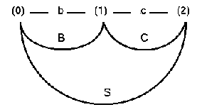
I would like to thank my major professor, Dr Michael A. Covington, for many useful suggestions and constant encouragement during my work. Thanks also to Dr Donald Nute and Dr Salikoko Mufwene for their constructive cooperation. Kevin Weinrich has worked his way through this thesis and gave many helpful hints regarding wording, style, and layout.
Since this thesis also marks the end of my studies at the University of Georgia, I want to use this opportunity to thank everyone who enabled me to spent these two inspiring years in Athens and everybody who helped to make it a pleasant time. Thanks go to the Fulbright Commission for providing the financial basis. Thanks also go to the staff of the ACMC at the University of Georgia for the office support and for providing the computer facilities. I would also like to thank everybody who gave moral support. In particular Ron Gonsher who was an always witty and considerate officemate and also Selim Nuri, my roommate, for many late-night philosophical discussions.
Finally I would like to thank all the friends back home in Germany whose letters over the years meant so much to me. Special thanks go to Irmtrud Kron for keeping me in touch with my home university and for her confidence in and support of my work. Last but foremost I owe appreciation to my father and to my sisters Birgit and Anke.
Athens, GA, May 1988.